The Bradley-Terry model is a powerful statistical tool for analyzing pairwise comparisons, widely used in sports analytics, consumer preference studies, and competitive rankings. This model estimates the probability of one item defeating another based on latent strength parameters, offering insights into relative abilities even when direct comparisons are incomplete. All of the models that can be found in DRatings use the Bradley-Terry method as the base formula. Let’s explore how it works and apply it to a hypothetical baseball league with six teams.
Understanding the Bradley-Terry Model
The model assigns each competitor (e.g., a baseball team) a strength parameter pi. The probability that team
i beats team j is given by:
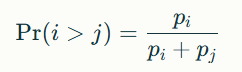
These parameters are typically estimated via maximum likelihood from historical matchup data. Higher pi values indicate stronger teams. The model can also be expressed in logit form, resembling logistic regression:
![]()
Example: Simulated Baseball League
Consider six teams (A–F) with the following head-to-head results from a 25-game season (each pair plays 5 games):
| A | B | C | D | E | F | Total Record | |
|---|---|---|---|---|---|---|---|
| A | 0 | 3 | 4 | 2 | 3 | 4 | 16-9 |
| B | 2 | 0 | 3 | 3 | 2 | 3 | 13-12 |
| C | 1 | 2 | 0 | 4 | 3 | 3 | 13-12 |
| D | 3 | 2 | 1 | 0 | 4 | 2 | 12-13 |
| E | 2 | 3 | 2 | 1 | 0 | 3 | 11-14 |
| F | 1 | 2 | 2 | 3 | 2 | 0 | 10-15 |
Step 1: Model Fitting
Here’s a complete R implementation of the Bradley-Terry model with proper normalization:
library(BradleyTerry2)

# Create matchup data
matchups <- data.frame(
  winner = c("A","A","A","A","A","B","B","B","B","C","C","C","D","D","E","F",
             ... ), # Full pairwise data
  loser = c("B","C","D","E","F","A","C","D","E","A","B","D","A","B","D","E","F", ... )
)

# Fit model
bt_model <- BTm(outcome = rep(1, nrow(matchups)),
                player1 = matchups$winner,
                player2 = matchups$loser)

# Get team strengths
strengths <- exp(BTabilities(bt_model)[,1])
Step 2: Estimated Strengths
The model outputs relative strengths (normalized to sum to 1):
| Team | Strength (pi) | Rank |
|---|---|---|
| A | 0.221 | 1 |
| B | 0.172 | 2 |
| C | 0.185 | 3 |
| D | 0.168 | 4 |
| E | 0.128 | 5 |
| F | 0.106 | 6 |
Step 3: Estimated Strengths
Using these strengths, we calculate the probability of Team A beating Team F:
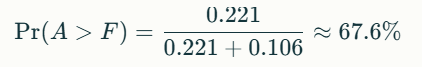
The 67.6% is not just a reflection of past win-loss records, but an estimate based on all pairwise results, accounting for the relative difficulty of each team’s schedule and their performance against all opponents. The model assumes that outcomes depend only on these strengths and are not influenced by other factors (like home field, injuries, or margin of victory). These factors are absolutely important and should be added to any sort of advanced model.
Conclusion
The Bradley-Terry model offers a clear and mathematically sound way to compare teams based on head-to-head results, translating raw win-loss data into meaningful probabilities. By estimating each team’s underlying strength, it not only ranks teams fairly but also predicts future matchups—like Team A’s 67.6% chance of beating Team F—with intuitive logic. Whether for sports analysis, tournament planning, or competitive ranking, the Bradley-Terry model is a powerful tool for turning game results into actionable insights.